Running HOS-NWT
HOS-NWT has been developed for command-line run with an input file containing all specifications needed (name can be arbitrary but will be referred to input_HOS-NWT.dat in the following for clarity). The following commands can be executed:
Linux environment (in a terminal):
./HOS-NWT input_HOS-NWT.dat
Windows environment (using the standard command prompt
cmd):
HOS-NWT.exe input_HOS-NWT.dat
Note
All output files will be created in a directory Results that has to be created before the run by the user.
Input file
The input file has the following form and is usually named input_HOS-NWT.dat. This subsection describes in details the content of the file.
---------------------- Tank dimensions -----------------------
Length(m) of the wavetank    :: xlen             :: 120.0d0
Beam(m) of the wavetank      :: ylen             :: 100.d0
Depth(m) of the wavetank     :: h                :: 5.d0
------------------------ Select case --------------------------
Choice of computed case      :: icase            :: 3
------------------ Sloshing case (icase = 1) ------------------
Number of the natural mode   :: islosh           :: 3
Amplitude (m) of the mode    :: aslosh           :: 0.2d0
--------------- Monochromatic case (icase = 2) ----------------
Amplitude (m) of wave train  :: amp_mono         :: 0.1d0
Frequency (Hz) of wave train :: nu_mono          :: 0.5588d0
Angle (deg) from x-axis      :: theta_mono       :: 0.d0
Phasis (rad) of wave train   :: ph_mono          :: 0.d0
Directional wmk type         :: ibat             :: 2
Wave target distance (ibat=3):: xd_mono          :: 18.d0
-------------------- File case (icase = 3) --------------------
Name of frequency file       :: file_name        :: Hs4_Tp10
Frequency cut-off            :: i_cut            :: 0
Low cut_off frequency (Hz)   :: nuc_low          :: 0.3d0
High cut_off frequency (Hz)  :: nuc_high         :: 3.d0
------------------ Irregular wave (icase=4) -------------------
Significant wave height (m)  :: Hs               :: 0.05d0
Peak period (s)              :: Tp               :: 1.d0
Shape factor (Jonswap)       :: gamma            :: 3.3d0
Seed number for random numb. :: iseed            :: 513
-------------------- Wavemaker definition ---------------------
Nonlinear order of wavemaker :: i_wmk            :: 2
Type (1: piston, 2: hinged)  :: igeom            :: 2
Rotation axis distance       :: d_hinge          :: 1.d0
Time ramp                    :: iramp            :: 0
Time ramp duration (s)       :: Tramp            :: 5.0d0
----------------------- Numerical beach -----------------------
Absorption numerical beach   :: iabsnb           :: 1
Beginning front num. beach   :: xabsf            :: 0.8d0
Absorption strength front    :: coeffabsf        :: 1.d0
------------- Elevation/Velocity-Pressure probes --------------
Use of probes                :: iprobes          :: 1
Filename of probe positions  :: pro_file         :: prob.inp
---------------------- Time-integration -----------------------
Duration of the simulation   :: T_stop           :: 50.0d0
Time tolerance: RK 4(5)      :: toler            :: 1.e-4
Output frequency             :: f_out            :: 30.d0
--------------------------- Output ----------------------------
Output: 1-dim. ; 0-nondim.   :: idim             :: 1
free surface plot            :: i3d              :: 0
modes plot                   :: imodes           :: 0
wavemaker motion plot        :: iwmk             :: 0
Swense output 1='yes',0='no' :: i_sw             :: 0
HDF5 output 1='yes',0='no'   :: is_hdf5          :: 0
----------------------- Discretization ------------------------
Number of points in x-dir.   :: n1               :: 512
Number of points in y-dir.   :: n2               :: 1
Number of points in y-dir.   :: n3               :: 17
HOS nonlinearity order       :: mHOS             :: 3
Dealiasing parameters in x   :: p1               :: 3
Dealiasing parameters in y   :: p2               :: 1
Filtering in x-direction     :: coeffiltx        :: 1.d0
Filtering in y-direction     :: coeffilty        :: 1.d0
Filtering in z-direction     :: coeffiltz        :: 1.d0
--------------------- Wave breaking type ---------------------
Breaking model type          :: ibrk             :: 0
---------- Tian model characteristics (ibrk=1 or 3) ----------
Breaking threshold           :: threshold        :: 0.85d0
alpha eddy_viscosity         :: alpha_eddy_vis   :: 0.02d0
Length ramp visc. (wrt Lc)   :: ramp_eddy        :: 0.25d0
Change of breaking length    :: fact_Lbr         :: 1.d0
Change of breaking duration  :: fact_Tbr         :: 1.d0
cubic spline interpolant     :: numspl           :: 5
Additional constant visc.    :: eqv_vis          :: 0.d0
-------- Chalikov model characteristics (ibrk=2 or 3) --------
Filter order                 :: order_filt       :: 1
Filter param                 :: r_filt           :: 0.75d0
Filter coefficient           :: coeffilt_chalikov:: 0.9d0
Diffusion strength           :: Cb               :: 0.03d0
Diffusion threshold          :: threshold_s      :: 75.d0
Tank dimension
xlenis the length (in m) of the wave tank (Lx in Fig. 2)ylenis the beam (in m) of the wave tank (Ly in Fig. 2, useful only in 3D)his the depth (in m) of the wave tank (constant)
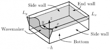
Fig. 2 Wave tank and coordinate system
Description of initial conditions
icase = 1: Sloshing caseComputation starts with a normal mode of the tank (in x-direction) of a given amplitude. It is defined by
islosh(mode number) andaslosh(amplitude in m)
icase = 2: Monochromatic caseRegular wave is generated in the NWT
User defines amplitude (
amp_monoin m), frequency (nu_monoin Hz), phase (ph_monoin rad)3D simulations uses in addition
theta_mono: the angle of propagation (in deg)ibat: the method used for directional wave generation. ibat=2 uses snake’s principle and ibat=3 uses Dalrymple’s methodxd_mono: uses the wave target distance (in m) for Dalrymple’s method (ibat=3)
icase = 3and31and32and33: File caseWavemaker movement is deduced from input file named ‘file_name’
Fine description wavemaker motion description in input files may be found in the Wavemaker motion from file section:
icase=3: file_name.dat describes the frequency components of wavemaker movement and file_name.cfg describes the configuration of wavemakericase=31: file_name.txt is an output of control software used in ECN Wave Basinicase=32: file_name.txt is an output of control software used in ECN Towing Tankicase=33: file_name.txt is an output of control software used in other tanks
i_cutspecifies if a frequency cut off is used (i_cut=1) or not. Latter is defined by lownuc_lowand highnuc_highcut-off frequencies (in Hz)
icase = 4and41: Irregular waveWavemaker movement creates an irregular wave field with a given Hs and Tp
icase = 4: JONSWAP spectrum withgammashape factoricase = 41: Bretschneider spectrum
iseeddefines the number used for random wave generation
Wavemaker definition
i_wmkdefines the order of non-linearity used for the wavemaker (recommended value is i_wmk=2 but it may be 1,2 or 3)igeomdefines the wavemaker vertical shape (1: piston, 2: hinged, see Fig. 3)d_hingedefines for hinged wavemaker the rotation axis distance (from bottom in m, d_hinge >= 0, see d in Fig. 3)irampspecifies the possible use of a time ramp on the wavemaker movement at the beginning of the simulation (iramp /= 0) and its shape (1: linear, 2: 2nd order polynom, 4: 4th order polynom)Trampis the duration (in s) of the time ramp on the wavemaker movement at the beginning of the simulation
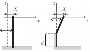
Fig. 3 Wavemaker shape: piston (igeom=1, left) and hinged (igeom=2, right)
Numerical beach
iabsnbdefines the use (iabsnb=1) or not (iabsnb=0) of numerical beach at the end of the tankxabsfdefines the location of the beginning of the numerical beach (ratio to the total length of wave tankxlen). The absorbing beach starts at x=xabsf*xlen.coeffabsfdefines the absorption strength of the previously defined numerical beach
Elevation/Velocity-pressure probes
iprobesdefines the possible use (iprobes /= 0) of probesiprobes=1: free-surface probes, each line gives location x (and y in 3D)iprobes=2: pressure probes, each line gives location x z (or x y z in 3D)
pro_filedefines the file name of probes position. In the input file example provided in Input file, it is named prob.inp
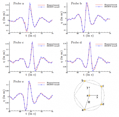
Fig. 4 Probe signals obtained for 3D focused wave
Time-integration
T_stopis the duration (in s) of the simulation (and of the wavemaker movement)tolergives the tolerance of the adaptative Runge-Kutta schemef_outgives the output frequency (in Hz) of the output files described in the following paragraph
Output files
Depending on the choices (0 to disable output) made in the input file (see Input file), different output files are created. They are created in a specific folder Results with a specific format dedicated to Tecplot visualization. Those are ASCII files that can be easily read with Python, Matlab, etc.
The parameter idim specifies if output are dimensional(=1) or nondimensional(=0).
3d.datgives the 3D free surface quantities (elevation η and surface velocity potential φs ) as function of time:i3d=1HOS_modes.datgives the modal amplitudes of free surface quantities (η and φs ) as function of time:imodes=1vol_energy.datgives the temporal evolution of volume and energywmk_motion.datgives the wavemaker motion as function of time:iwmk=1probes.datgives the free surface elevation at specific locations given in the file specified inpro_file:i_prob=1modes_HOS_SWENSE.datgives the file containing modal information of volumic HOS field for visualization, physical interpretation of wavefield, or possible coupling between HOS and wave-structure interactions model (see the dedicated package for coupling Grid2Grid): see post-processing section:i_sw=1
Those are standard outputs in ASCII format. The parameter is_hdf5 allows the use of HDF5 format instead of ASCII (for instance for data size concerns).
Note
HDF5 outputs requires the code to be compiled with the dedicated option (see corresponding section)
Note
MPI outputs are slightly modified for the files describing 3D spatial or modal quantities. Each computational core will output the spatial/modal part it has in memory. For instance the output file 3d.dat will be replaced in the case of HOS-NWT compiled with MPI and executed with 4 processes by 3d_000.dat, 3d_001.dat, 3d_002.dat, and 3d_003.dat files
Numerical parameters
n1is the number of spatial points (or equivalently modes) used in the x-directionn2is the number of spatial points (or equivalently modes) used in the y-direction. For a 2D simulation, choose n2=1n3is the number of spatial points (or equivalently modes) used in the z-direction, to describe the wave maker motionmHOSis the HOS order of nonlinearityp1describes the methodology used for dealiasing in x-direction. For total dealiasing p1=mHOS should be used while for partial dealiasing, one should use p1<mHOSp2describes the methodology used for dealiasing in y-direction. For total dealiasing p2=mHOS should be used while for partial dealiasing, one should use p2<mHOS. For a 2D simulation, choose p2=1coeffiltxparameterizes a possible filtering along x-direction. The mode numbers in the range [coeffiltx;1]*n1 are set to zerocoeffiltyparameterizes a possible filtering along y-direction. The mode numbers in the range [coeffilty;1]*n2 are set to zerocoeffiltzparameterizes a possible filtering along x-direction. The mode numbers in the range [coeffiltz;1]*n3 are set to zero
Note
The user needs to choose the numerical parameters wisely to achieve accurate numerical solution. Some elements are provided in corresponding section
Wave breaking model
The end of the input file is dedicated to the parametrization of the wave breaking models.
Warning
The breaking models are only implemented for unidirectional waves for now (n2=1)
ibrkdefines the use of the wave breaking models in HOS-NWTibrk=0: no model for wave breaking (original HOS-NWT solver)ibrk=1: Barthelemy’s model for breaking onset and Tian’s model for the dissipation, see [Seiffert et al., 2017, Seiffert and Ducrozet, 2018]:ibrk=2: Chalikov’s breaking model for the breaking onset and dissipation, see [Seiffert and Ducrozet, 2017]:ibrk=3: Combined use of previous models (ibrk=1 and ibrk=2)
Barthelemy-Tian model parameters are the following (ibrk=1 and ibrk=3)
thresholdstands for the threshold used in Barthelemy breaking onset, which is the ratio of fluid velocity on phase velocity (default is 0.85)alpha_eddy_visstands for the eddy viscosity used in Tian’s dissipation model (default is 0.02)ramp_eddystands for the length (with respect to crest length) of the spatial ramp used to apply eddy viscosity (default is 0.25)fact_Lbrcan be used to increase the dissipation length parameterized in Tian’s model (default is 1.0)fact_Tbrcan be used to increase the dissipation duration parameterized in Tian’s model (default is 1.0)numsplstands for the spline interpolant used to refine the HOS grid for better estimate of crest speed (default is 5)eqv_visstands for a constant additional viscosity added to the whole spatial domain (default is 0.0)
Chalikov model parameters are the following (ibrk=2 and ibrk=3)
order_filtstands for the exponent applied to the maximum wavenumber in hyperviscous filter continuously applied in Chalikov’s model (default 1.0)r_filtdefines the constant parameter of the hyperviscous filter continuously applied in Chalikov’s model (default 0.25)coeffilt_chalikovdefines the application of the hyperviscous filter. The latter starts is applied on mode numbers in [coeffilt_chalikov,1]*n1Cbstands for the strength of the dissipation applied in Chalikov’s model (default 0.05). This multiplies the curvature of the free surfacethreshold_sstands for the threshold used in Chalikov’s model for breaking onset, based on the curvature of the free surface (default 10.0)
Examples
Some input files examples are available in the Benchmark directory. See Benchmark cases for details.
Important notice
For irregular wave motion (i.e. icase=3, 31, 32, 33, 4 or 41), the description of wavemaker motion is filtered above a cut-off limit of 4 Hz. In usual test cases, this is not a problem since HOS-NWT is dedicated to the generation and propagation of gravity waves (no capillary effects taken into account): waves with frequencies higher than 4 Hz could not be considered pure gravity waves. However, this may be changed in wavemaking_HOS.f90file for specific purpose.